Planet CLAM is a window into
the world, work and lives of
CLAM hackers and contributors.
The planet is open to any blog feed that
occasionally relates with CLAM or its brother projects
like testfarm.
Ask in the devel list to get in.
There have recently been some articles (e.g. This list of influencers) that have pointed to this blog and lamented that I don't update it regularly anymore. It is true. I now realize I should have at least posted something here to direct readers to the places where I keep posting in case they find I might have something interesting to say.
First and foremost, given that I joined Quora about a year ago, I have been using the Quora product itself to post most of my writing. You can find my profile here. I have found that I can reformulate almost anything I want to say in the form of an answer to a Quora question. Besides, my posts there get a ton of views (I am almost about to reach 2 million views in about a year) and good interactions. Also, I have written some posts in the Quora Engineering Blog describing some of our work.
I also keep very active on Twitter, and every now and then I will update my LinkedIn with some professional posts.
Recently, I gave Medium a try. I am not really sure how often I will update my blog there, but I am almost certain that my Medium blog will take precedence over this one. Medium is indeed a much better blogging platform than Blogger.
So, yes, I guess this is a farewell to Technocalifornia unless every now and then I decide to simply post a collection of posts elsewhere just to make sure that people visiting this blog don't get the sense that I am not active anymore. Let me know if you feel that would be interesting for you.
(This is a blogpost version of a talk I gave at MLConf SF 11/14/2014. See below for original video and slides)
There are many good textbooks and courses where you can be introduced to machine learning and maybe even learn some of the most intricate details about a particular approach or algorithm (See my answer on Quora on what are good resources for this). While understanding that theory is a very important base and starting point, there are many other practical issues related to building real-life ML systems that you don’t usually hear about. In this post I will share some of the most important lessons learned in years of building large-scale ML solutions that power products such as Netflix and scale to millions of users across many countries.
And just in case it doesn't come across clearly enough, let me insist on this once again: it does pay off to be knowledgeable and have deep understanding of the techniques and theory behind classic and modern machine learning approaches. Understanding how Logistic Regression works or the difference between Factorization Machines and Tensor Factorization, for example, is a necessary starting point. However, this in itself might not be enough unless you couple it with the real-life experience of how these models interact with systems, data, and users in order to obtain a really valuable impact. The next ten lessons are my attempt at trying to capture some of that practical knowledge.
1. More Data vs. and Better Models
A lot has been written about whether the key to better results lays in improving your algorithms or simply on throwing more data at your problem (see my post from 2012 discussing this same topic, for example).
In the context of the Netflix Prize, Anand Rajaraman took an early stand on the issue by claiming that "more data usually beats better algorithms". In his post he explained how some of his students had improved some of the existing results on the Netflix ratings dataset by adding metadata from IMDB.
Fig 1. More data usually beats better algorithms
Although many teams in the competition tried to follow that lead and add extra features to improve results, there was little progress in that direction. As a matter of fact, just a year later some of the leaders of what would become the runner up team published a paper in which they showed that adding metadata had very little impact in improving the prediction accuracy of a well-tuned algorithm. Take this as a first example of why adding more data is not always the solution.
Fig 2. Even a Few Ratings Are More Valuable than Metadata
Of course, there are different ways to "add more data". In the example above we were adding data by increasing the number and types of features, therefore increasing the dimensionality of our problem space. We can think about adding data in a completely different way by fixing the space dimensionality and simply throwing more training examples at it. Banko and Brill showed in 2001 that in some cases very different algorithms responded equally well by improving to more training data (see figure below)
Fig 3. Banko and Brill's "famous" model performance curves
Google's Research Director and renowned AI figure Peter Norvig is quoted as saying that "Google does not have better algorithms, just more data". In fact, Norvig is one of the co-authors of "The Unreasonable Effectiveness of Data" where in a similar problem to the one in Banko and Brill (language understanding) they also show how important it is to have "more data".
Fig 4. The Unreasonable Effectiveness of Data
So, is it true that more data in the form of more training examples will always help? Well, not really. The problems above are complex models with a huge number of features which lead to situations of "high variance". But, in many other cases this might not be true. See below for example a real-case scenario of an algorithm in production at Netflix. In this case, adding more than 2 million training examples has very little to no effect.
Fig 5. Testing Accuracy of a real-life production model
So, this leads to our first lesson learned, which in fact will expand over several of the following ones: it is not about more data versus better algorithms. That is a false dichotomy. Sometimes you need more data, and sometimes you don't. Sometimes you might need to improve your algorithm and in others it will make no difference. Focusing exclusively on one or the other will lead to far from optimal results.
2. You might not need all your "Big Data"
This second lesson is in fact a corollary of the previous one, but I feel it is worth to mention explicitly on its own. It seems like nowadays everyone needs to make use of all their "Big Data". Big Data is so hyped that it seems like if you are not using huge quantities of data you must be doing something wrong. The truth though, as discussed in lesson 1, is that there are many problems for which you might be able to get similar results by using much less data than the one you have available. Think for example of the Netflix Prize where you had 0.5 Million users in the dataset. In the most favored approach, the data was used to compute a Matrix of 50 factors. Would the result change much if instead of the 0.5 M users you used, say 50 Million? Probably not. A related, and important, question is how do you determine what subset of your data to use. A good initial approach would be to random sample your original data to obtain as many samples you need for your model training. That might not be good enough though. Staying with the Netflix Prize example, users might be very different and not homogeneously distributed in our original population. New users, for example, will have much fewer ratings and increase sparsity in the dataset. On the other hand, they might have a different behavior from more tenured users and we might want to make our model capture it. The solution is to use some form of stratified sampling. Setting up a good stratified sampling scheme is not easy since it requires us to define the different strata, and decide what is the right combination of samples for the model to learn. However, as surprising as it might sound, a well-defined stratified sampled subset might accomplish even better results than the original complete dataset. Just to be clear, I am not saying that having lots of data is a bad thing, of course it is not. The more data you have, the more choices you will be able to make on how to use it. All I am saying is that focusing on the "size" of your data versus the quality of the information in the data is a mistake. Garner the ability to use as much data as you can in your systems and then use only as much as you need to solve your problems.
3. The fact that a more complex Model does not improve things does not mean you don't need one
Imagine the following scenario: You have a linear model and for some time you have been selecting and optimizing features for that model. One day you decide to try a more complex (e.g. non-linear) model with the same features you have been engineering. Most likely, you will not see any improvement.
After that failure, you change your strategy and try to do the opposite: You keep the old model, but add more expressive features that try to capture more complex interactions. Most likely the result will be the same and you will again see little to no improvements. So, what is going on? The issue here is that simply put more complex features require a more complex model, and vice versa, a more complex model may require more complex features before showing any significant improvement. So, the lesson learned is that you must improve both your model and your feature set in parallel. Doing only one of them at a time might lead to wrong conclusions.
4. Be thoughtful about how you define your training/testing data sets
If you are training a simple binary classifier, one of the first tasks to do is to define your positive and negative examples. Defining positive and negative labels for samples though may not be such a trivial task. Think about a use case where you need to define a classifier to distinguish between shows that users watch (positives) and do not watch (negatives). In that context, would the following be positives or negatives?
User watches a movie to completion and rates it 1 star
User watches the same movie again (maybe because she can’t find anything else)
User abandons movie after 5 minutes, or 15 minutes… or 1 hour
User abandons TV show after 2 episodes, or 10 episode… or 1 season
User adds something to her list but never watches it
As you can see, determining whether a given example is a positive or a negative is not so easy. Besides paying attention to your positive and negative definition, there are many other things you need to make sure to get right when defining your training and testing datasets. One such issue is what we call Time Travelling. Time traveling is defined as usage of features that originated after the event you are trying to predict. E.g. Your rating a movie is a pretty good prediction of you watching that movie, especially because most ratings happen AFTER you watch the movie. In simple cases as the example above this effect might seem obvious. However, things can get very tricky when you have many features that come from different sources and pipelines and relate to each other in non-obvious ways. Time traveling has the effect of increasing model performance beyond what would seem reasonable. That is why whenever you see an offline experiment with huge wins, the first question you might want to ask yourself is: “Am I time traveling?”. And, remember, Time Traveling and positive/negative selection are just two examples of issues you might encounter when defining your training and testing datasets. Just make sure you are thoughtful about how you define all the details of your datasets.
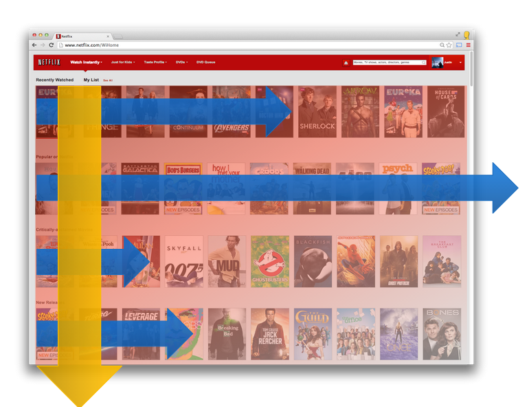
5. Learn to deal with (the curse of) the Presentation Bias
Fig 6. Example of an Attention Model on a page
Let's face it, users can only click and act on whatever your algorithm (and other parts of your system) has decided to show them. Of course, what your algorithm decided to show is what it predicted was good for the user. Let's suppose that a new user comes in and we decide to show the user only popular items. The fact that a week later the user has only consumed popular items does not mean that's what the user like. That's the *only* thing she had a chance to consume! As many (including myself) have mentioned in the past, is important to take that into account in your algorithms and try to somehow break this "Curse of the Presentation Bias". Most approaches to addressing this issue are based on the idea that you should "punish" items that were showed to the user but not "clicked on". One way to do so is by implementing some presentation discounting mechanism (see this KDD 2014 paper by the LinkedIn folks). Another way to address the issue is to use viewed but not clicked items as negatives in your training process. This, in principle, makes sense: if a user searched for a query and ended up clicking in result number three it means the first two results were bad and should be treated as negatives... or not? The problem with this is that although the first two items were likely worse than the third one (at least in that particular context), this does not mean they were any worse than item in position 4, let alone item in position 5000, which your original model decided was no good at all. Yes, you want to remove the presentation bias, but not all of it since it responds to some hopefully well-informed decisions your model took in the first place. So, what can we do? First thing that comes to mind is to introduce some sort of randomization in the original results. This randomization should allow to collect unbiased user feedback so as to whether those items are good or not (see some of the early publications by Thorsten Joachims such as this one or take a look at the idea of result dithering proposed by Ted Dunning). Another better approach is to develop some sort of "attention model" of the user. In this case both clicked and non-clicked items will be weighted by the probability that the user noticed them in the first place depending on their location on the page (see some of the recent work by Dmitry Lagun for interesting ideas on this area. Finally, yet another and well established way to address presentation bias is by using some sort of explore/exploit approach, in particular multi-armed bandits. By using a method such as Thompson Sampling, you can introduce some form of "randomization" on the items that you are still not sure about, while still exploiting as much as you can from what you already know for sure (see Deepak Argawal's Explore/Exploit approach to recommendations or one of the many publications by Thorsten Joashims for more details on this).
6. The UI is the only communication channel between the Algorithm and what matters most: the Users
Fig 7. The UI is the algorithm's connection point with the user
From the discussion in the previous lesson it should be clear by now how important it is to think about the presentation layer and the user interface in our machine learning algorithmic design. On the one hand, the UI generates all the user feedback that we will use as input to our algorithms. On the other hand, the UI is the only place where our algorithms will be shown. It doesn't matter how smart our ML algorithm is. If the UI hides its results or does not give the user the ability to give some form of feedback, all our efforts on the modeling side will have been in vain. Also, it is important to understand that a change in the user interface might require a change in the algorithms and vice versa. Just as we learned before that there is an intimate connection between features and models, there is also another to be aware of between the algorithms and the presentation layer.
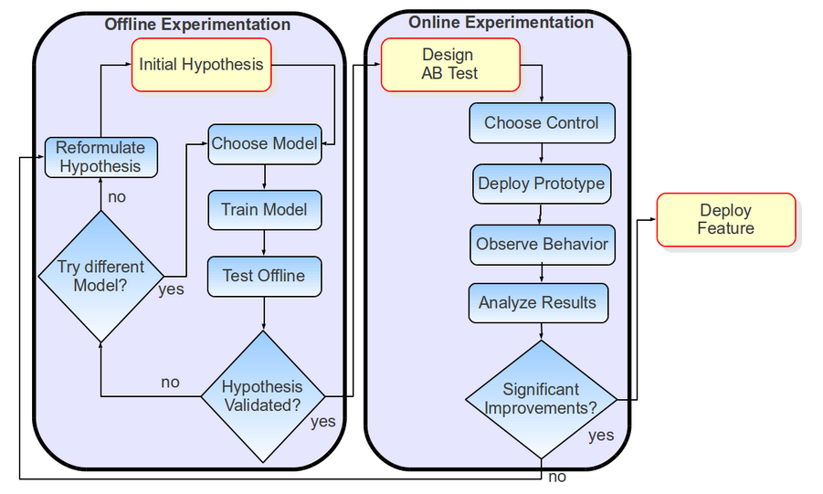
7. Data and Models are great. You know what is even better? The right evaluation approach.
Fig 8. Offline/Online Innovation Approach
This is probably one of the most important of the lessons in this post. Actually, as I write this I feel that it is a bit unfortunate that this lesson might seem as "just another lesson" hidden in position 7. This should be a good place to stress that these lessons in this post are not sorted from more to less important, they are just grouped in topics or themes. So, yes, as important as all the other discussions about data, models, and infrastructure may be, they are all rather useless if you don't have the right evaluation approach in place. If you don't know how to measure an improvement you might be endlessly spinning your wheels without really getting anywhere. Some of the biggest gains I have seen in practice have indeed come from tuning the metrics to which models were being optimized. Ok, then what is the "right evaluation approach"? Figure 8 illustrates an offline/online approach to innovation that should be a good starting point. Whatever the final goal of your machine learning algorithm is in your product you should think of driving your innovation in two distinct ways: offline and online.
Fig 9. Offline Evaluation
First, you should generate datasets that allow to try different models and features in an offline fashion by following a traditional ML experimentation approach (see Figure 9): You train your model to a training seat, you probably optimize some (hyper)parameters to a validation set, and finally measure some evaluation metrics on a test set. The evaluation metrics in our context are likely to be IR metrics such as precision and recall, ROC curves, or ranking metrics such as NDCG, MRR, or FPC (Fraction of Concordant Pairs). Note though that the selection of the metric itself has its consequences. Take a look at Figure 10 for an example of how the different ranking metrics weight different ranks being evaluated. In that sense, metrics such as MRR or (especially) NDCG will give much more importance to the head of the ranking, while FPC will be weighting more on the middle of the ranks. The key here is that depending on your application you should choose the right metric.
Fig. 10. Importance given to different ranks by typical ranking metrics
Offline experimentation is great because once you have the right data and the right metric it is fairly cheap to run many experiments with very few resources. Unfortunately, a successful offline experiment can only be generally used as an indication of a promising approach worth testing online. While most companies are investing in finding better correlation between offline and online results, this is still, generally speaking, an unsolved issue that deserves more research (see this KDD 2013 paper, for example). In online experimentation the most usual approach is to do A/B testing (other approaches such as Multiarmed Bandit Testing or Interleaved Testing are becoming more popular recently but are beyond the scope of this post). The goal of an A/B test is to measure difference in metrics across statistically identical populations that each experience a different algorithm. As with the offline evaluation process, and perhaps even more here, it is very important to choose the appropriate evaluation metric to make sure that most if not all decisions on the product are data driven. Most people will have a number of different metrics they are tracking in any AB test, but it is important to clearly identify the so-called Overall Evaluation Criteria (OEC). This should be the ultimate metric used for product decisions. In order to avoid noise and make sure the OEC maps well to business success it is better to use a long-term metric (e.g. customer retention). Of course, the issue with that is that you need time, and therefore resources, to evaluate a long-term metric. That is why it is very useful to have short-term metrics that can be used as initial early reads on the tests in order to narrow down worthwhile hypothesis that need to wait until the OEC read is complete.
If you want more details on the online experimentation piece there are many good reads, starting with the many good articles by Bing's Ronny Kohavi (see this, for example).
8. Distributing algorithms? Yes, but at what level?
There always comes a time in the life of a Machine Learning practitioner when you feel the need to distribute your algorithm. Distributing algorithms that require of many resources is a natural thing to do. The issue to consider is at what *level* does it make sense to distribute. We distinguish three levels of distribution:
Level 1. For each independent subset of the overall data
Level 2. For every combination of the hyperparameters
Level 3. For all partitions in each training dataset
In the first level we may have subsets of the overall data for which we need to (or simply can) train an independently optimized model. A typical example of this situation is when we opt for training completely independent ML models for different regions in the world, different kinds of users, or different languages. In this case, all we need to do is to define completely independent training datasets. Training can then be fully distributed requiring no coordination or data communication.
In the second level, we address the issue of how to train several models with different hyperparameter values in order to find the optimal model. Although there are smarter ways to do it, let's for now think of the worst-case grid search scenario. We can definitely train models with different values of the hyperparameters in a completely distributed fashion, but the process does require coordination. Some central location needs to gather results and decide on the next "step" to take. Level 2 requires data distribution, but not sharing since each node will use a complete replica of the original dataset and the communication will happen at the level of the parameters.
Finally, in level 3 we address the issue of how to distribute or parallelize model training for a single combination of the hyperparameters. This is a hard problem, but there has been a lot of research put into it. There are different solutions with different pros and cons. You can distribute computation over different machines splitting examples or parameter using, for example, ADMM. Recent solutions such as the Parameter Sever promise to offer a generic solution to this problem. Another option is to parallelize on a single multicore machine using algorithms such as Hogwild. Or, you can use the massive array of cores available in GPU cards.
As an example of the different approaches you can take to distribute each of the levels, take a look at what we did in our distribution of Artificial Neural Networks over the AWS cloud (see Figure 11 below for an illustration). For Level 1 distribution, we simply used different machine instances over different AWS regions. For Level 2 we used different machine in the same region and a central node for coordination. We used Condor for cluster coordination (although other options such as StarCluster, Mesos, or even Spark) are possible. Finally, for level 3 optimization, we used highly optimized CUDA code on GPUs.
Fig 11. Distributing ANN over the AWS cloud
9. It pays off to be smart about your Hyperparameters
As already mentioned in the previous lesson, one of the important things you have to do when building your ML system is to tune your hyperparameters. Most, if not all, algorithms will have some hyperparameters that need to be tuned: learning rate in matrix factorization, regularization lambda in logistic regression, number of hidden layers in a neural network, shrinkage in gradient boosted decision trees... These are all parameters that need to be tuned to the validation data. Many times you will face situations in which models need to be periodically retrained and therefore hyperparameters need to be at least fine-tuned. This is a clear situation where you need to figure out a way to automatically select the best hyperparameters without requiring a manual check. As a matter of fact, having an automatic hyperparameter selection approach is worthwhile even if all you are doing is the initial experimentation. A fair approach is to try all possible combinations of hyperparameters and pick the one that maximizes a given accuracy metric on the validation set. While this is, generally speaking, a good idea, it might be problematic if implemented directly. The issue is that blindly taking the point that optimizes whatever metric does not take into account the possible noisiness in the process and the metric. In other words, we can't be sure that if point A has an accuracy that is only 1% better than point B, point A is a better operating point than B. Take a look at Figure 12 below, which illustrates this issue by showing (made up) accuracy results for a model given different values of the regularization parameter. In this particular example the highest accuracy is for no regularization, plus there is a relatively flat plateau region for values of lambda between 0.1 and 100. Blindly taking a value of lambda of zero is generally a bad idea since it points to overfitting (yes, this could be checked by using the test dataset). But, beyond that, going to the "flat region", is it better to stick with the 0.1 value? By looking at the plot I would be inclined to take 100 as the operating point. This point is (a) non-zero, and (b) noise-level different in terms of accuracy from the other non-zero values. So, one possible rule of thumb to use is to keep the highest non-zero value that is noise level different in terms of the optimizing metric from the optimal point.
Fig 12. Example of model accuracy vs. regularization lambda
I should also add that even though in this lesson I have dsf about using a brute-force grid search approach to hyperparameter optimization, there are much better things you can do which are again beyond the scope of this post. If you are not familiar with Bayesian Optimization, start with this paper or take a look at Spearmint or MOE.
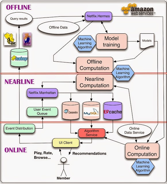
10. There are things you can do Offline and there are things you can't... and there is Nearline for everything in between
In the lessons so far we have talked about the importance of data, models, UI, metrics... In this last lesson I thought it was worth to focus on systems and architecture. When the final goal of your ML model is to have impact on a product, you are necessarily going to have to think about the right system architecture. Figure 13 depicts a three level architecture that can be used as a blueprint for any machine learning system that is designed to have a customer impact. The basic idea is that it is important to have different layers in which to trade off latency vs. complexity. Some computations need to be as real-time as possible to quickly respond to user feedback and context. Those are better off in an online setting. On the other extreme, complex ML models that require large amounts of data and lengthy computations are better done in an offline fashion. Finally, there is a Nearline world where operations are not guaranteed to happen in real-time but a best effort is performed to do them as "soon as possible".
Fig 13. This three level architecture can be used as a blueprint for machine learning systems that drive customer impact.
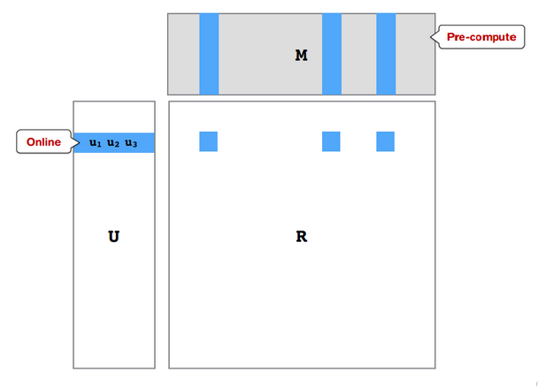
Interestingly, thinking about these three "shades of latency" also helps breaking down traditional machine learning algorithms into different components that can be executed in different layers. Take matrix factorization as an example. As illustrated in Figure 14, you can decide to do the more time-consuming item factor computation in an offline fashion. Once those item factors are computed, you can compute user factors online (e.g. solving a closed-from least squares formulation) in a matter of milliseconds in an online fashion.
Fig 14. Decomposing matrix factorization into offline and online computation
If you are interested in this topic take a look at our original blog post in the Netflix tech blog.
Conclusions
The ten lessons in this post illustrate knowledge gathered from building impactful machine learning and general algorithmic solutions. If I had to summarize them in 4 short take away messages those would probably be:
Be thoughtful about your data
Understand dependencies between data and models
Choose the right metric
Optimize only what matters
I hope they are useful to other researchers and practicioners. And, would love to hear about similar or different experiences in building real-life machine learning solutions in the comments. Looking forward to the feedback.
Acknowledgments
Most of the above lessons have been learned in close collaboration with my former Algorithms Engineering team at Netflix. In particular I would like to thank Justin Basilico for many fruitful conversations, feedback on the original drafts of the slides, and for providing some of the figures in this post.
A couple of weeks ago, I gave a 4 hour lecture on Recommender Systems at the 2014 Machine Learning Summer School at CMU. The school was organized by Alex Smola and Zico Kolter and, judging by the attendance and the quality of the speakers, it was a big success.
This is the outline of my lecture:
Introduction: What is a Recommender System
“Traditional” Methods
Collaborative Filtering
Content-based Recommendations
"Novel" Methods
Learning to Rank
Context-aware Recommendations
Tensor Factorization
Factorization Machines
Deep Learning
Similarity
Social Recommendations
Hybrid Approaches
A practical example: Netflix
Conclusions
References
You can access the slides in Slideshare and the videos in Youtube, but I thought it would make sense to gather both here and link them together.
Last week,
python-wavefile
received a pull request from the PyDAW project
to make it compatible with Python3.
So, I awaked the project to pull the contributions and addressing some of the old pending tasks.
I did not realize python-wavefile
got more relevance than most of my github projects:
Other people, not just me, are actually using it, and that’s cool.
So I think I owe the project a blog entry… and maybe a logo.
python-wavefile is a Python module to read and write audio files in a pythonic way.
Instead of just exposing the C API of the powerful Eric De Castro Lopo’s libsndfile,
it enables common Python idioms and numpy bridging for signal processing.
There are many Python modules around wrapping libsndfile including an standard one.
At the end of the article I do a quick review of them and justify why i did yet-another libsndfile Python wrapper.
History
This module was born to cover the needs I had while doing research for my PhD thesis on 3D audio.
I needed
floating point samples and
multi-channel formats for Higher Order Ambisonics and multi-speaker mix-down.
I also needed efficient block processing,
as well as the inefficient, but sometimes convenient, Matlab-like load-it-all functionality.
This is why I proposed Xavi Serra, when he was starting
his Master Thesis,
a warm-up exercise:
Mocking up Python bindings for the libsndfile library using different methods:
Cython, CPython module, Boost, CTypes, SIP…
That exercise resulted in several mock-ups for each binding method,
and an almost full implementation using CPython,
based on the double layer strategy Xavi finally used for iPyCLAM:
A lower narrow layer making the C API available to Python as is, and a user layer adding the Python sugar.
As we evolved the wrapper towards the user layer we wanted,
CPython code became too complex.
So I created python-wavefile by reimplementing the user API
we defined with Xavier Serra but relying on the C-API wrapping
defined in libsndfile-ctypes.
Python-wave, the official API and the root of all evil
Why do we do that?
The root of all evil is Python official module to deal with wave files.
It is based on libsndfile as well, but the Python API is a crap, a real crap:
:-) As standard lib it is available on every Python install, but…
:-( It has nasty accessors like getcomptype, getsampwidth…
Names with a hard to read/remember combination of shorts
Using getters instead of properties
:-( It just opens WAV files, and none of the many formats libsndfile supports
On writting, users are responsable of encoding samples which is a low level and error prone task.
Even worse, on reading, users have to implement decoding for every kind of encoding available.
Libsndfile actually does all this stuff for you, so why the hell to use the raw interface?
:-( It ignores Python constructs and idioms:
Generators to access files progressively in iterations
Context managers to deal safely with file resources
Properties instead of getters and setters
:-( It allocates a new data block for each block you read, which is a garbage collector nightmare.
:-( It has no support for numpy
A core lib cannot have a dependency on numpy but it is quite convenient feature to have to perform signal processing
Because of this, many programmers built their own libaudiofile wrapper
but most of them fail for some reason, to fulfill the interface I wanted.
Instead of reinventing the wheel I reused design and even code from others.
At the end of the article I place an extensive list of such alternatives and their strong and weak points.
The API by example
Let’s introduce the API with some examples.
To try the examples you can install the module from PyPi repositories using the pip command.
$ pip install wavefile
Notes for Debian/Ubuntu users:
Use sudo or su to get administrative rights
If you want to install it for Python3 use pip3 instead
Writting example
Let’s create an stereo OGG file with some metadata and a synthesized sound inside:
fromwavefileimportWaveWriter,FormatimportnumpyasnpwithWaveWriter('synth.ogg',channels=2,format=Format.OGG|Format.VORBIS)asw:w.metadata.title="Some Noise"w.metadata.artist="The Artists"data=np.zeros((2,512),np.float32)forxinxrange(100):# Synthesize a kind of triangular sweep in one channeldata[0,:]=(x*np.arange(512,dtype=np.float32)%512/512)# And a squared wave on the otherdata[1,512-x:]=1data[1,:512-x]=-1w.write(data)
Playback example (using pyaudio)
Let’s playback a command line specified audio file and see its metadata and format.
importpyaudio,sysfromwavefileimportWaveReaderp=pyaudio.PyAudio()withWaveReader(sys.argv[1])asr:# Print infoprint"Title:",r.metadata.titleprint"Artist:",r.metadata.artistprint"Channels:",r.channelsprint"Format: 0x%x"%r.formatprint"Sample Rate:",r.samplerate# open pyaudio streamstream=p.open(format=pyaudio.paFloat32,channels=r.channels,rate=r.samplerate,frames_per_buffer=512,output=True)# iterator interface (reuses one array)# beware of the frame size, not always 512, but 512 at leastforframeinr.read_iter(size=512):stream.write(frame,frame.shape[1])sys.stdout.write(".");sys.stdout.flush()stream.close()
Processing example
Let’s process some file by lowering the volume and changing the title.
reusing such block for each read and thus reducing the memory overhead, and
returning a slice of it when the last incomplete block arrives.
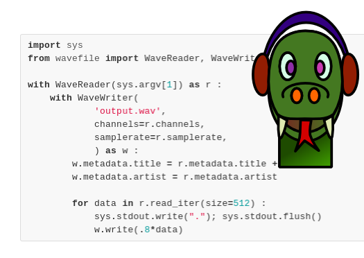
Masochist example
If you like you can still do things by hand using a more C-ish API:
importsys,numpyasnpfromwavefileimportWaveReader,WaveWriterwithWaveReader(sys.argv[1])asr:withWaveWriter('output.wav',channels=r.channels,samplerate=r.samplerate,)asw:w.metadata.title=r.metadata.title+" (masochist)"w.metadata.artist=r.metadata.artistdata=r.buffer(512)# equivalent to: np.empty((r.channels,512), np.float32, order='F')nframes=r.read(data)whilenframes:sys.stdout.write(".");sys.stdout.flush()w.write(.8*data[:,:nframes])nframes=r.read(data)
Notice that with read you have to reallocate the data yourself,
the loop structure is somewhat more complex with duplicated read inside and outside the loop.
You also have to slice to the actual number of read frames since
the last block usually does not have the size you asked for.
The API uses channel as the first index for buffers.
This is convenient because usually processing splits channels first.
But audio files (WAV) interleaves samples for different channels in the same frame:
f1ch1f1ch2f2ch1f2ch2f3ch1f3ch2...
Reads are optimized by using a read buffer with Fortran order (F).
Numpy handles the indexing transparently but for the read buffer,
and just for the read buffer we recommend to use the buffer() method.
That’s not needed for the rest of buffers, for example, for writting
and you don’t have to worry at all if you are using the read_iterAPI.
Load and save it all interface
This interface is not recommended for efficient processing,
because it loads all the audio data in memory at once,
but is sometimes convenient in order to have some code quickly working.
That was the pull request from Jeff Hugges of the PyDAW project.
Thanks a lot for the patches!
We managed to make Python 3 code to be also compatible with Python 2.
So now the same code base works on both versions and passes the same tests.
Unicode in paths and tags
Besides Python3 compatibility, now the API deals transparently with Unicode strings
both for file names and text tags such as title, artist…
If you encode the string before passing it to the API, and pass it as a byte string,
the API will take that encoding with no question and use it.
More safe is just passing the unicode string (unicode in Py2 and str in Py3).
In that case the API encodes or decodes the string transparently.
In the case of filenames, it uses the file system default encoding available to Python as sys.getfilesystemencoding().
In the case of text tags, it will use UTF-8 which is the standard for Vorbis based files (ogg, flac…).
WAV’s and AIFF standard just specifies about ASCII strings and I had my concerns about using UTF-8 there.
After a discussion with Eric de Castro,
we settled that UTF-8 is a safe option for reading and a nice one to push as de facto standard,
but I am still not confident about the later.
The alternative would have been raise a text encoding exception whenever a non ASCII character is written
to a WAV/AIFF.
I am still open to further arguments.
Seek, seek, seek
I also added API to seek within the file.
This enables a feature a user asked like reseting the file reading and being able to loop.
I was uncertain about libsndfile behaviour on seek.
Now such behaviour is engraved on API unit tests:
Seeks can be a positive or negative number of frames from a reference frame
Frames are as many samples as channels, being a sample a digitally encoded audio level
The reference point for the seeking can be the beginning (SET), the end (END) or the current next sample to be read (CUR)
That is, if your last read was a 10 frame block starting at 40, your current seek reference is 50
Seek returns the new frame position to be read if the jump is successful or -1 if not.
Jumps to the first frame after the last frame do not fail, even though that frame does not exist.
:-) Property accessors for format metadata and strings
:-( Not inplace read (creates an array every block read)
:-) No property accessors for strings
:-( No generator idiom
:-( Windows only setup
:-( Text tags not as properties
:-( Long access to constants (scoping + prefixing)
:-( Single object mixing read and write API’s
python-wavefile
That’s the one. I used the implementation layer from libsndfile-ctypes.
I really liked the idea of having a direct C mapping without
having to compile a CPython module,
and how nicely the numpy arrays were handled by CTypes.
Then, over that implementation layer,
I added a user level API implementing pythonic interface
including those supported by other wrappers and the new ones.
Many posts in this blog talk about WiKo, Hyde, pandoc…
Solutions we can use to edit wiki like pages as plain text files,
so that I can edit them with my preferred editor (vim),
do site wide search and replace,
track revisions using a version control system such subversion or git,
and reuse the same content to generate multiple media: pdf documents, web pages…
After that Grial Quest I have some solutions that works for me.
Indeed I am writting this entry using MarkDown which turns into a web page by means of Hyde.
But, meanwhile, some of the projects I am involved in already use some kind of traditional wiki system,
and most of them use Mediawiki.
Lucky for me,
this week, I have come across a useful git extension.
It git clones the content of a Mediawiki site as it were a git remote repository
so that you can pull revisions into your hard drive,
edit them and push them back into the wiki.
Cloning, pulling and pushing are slow.
Those are the operations that interact with the remote MediaWiki.
All the revision handling intelligence happens at users computer,
so git-mediawiki has to download a lot of information from mediawiki previously to do any action.
MediaWiki API entry points are not designed with those use cases in mind.
Supages do not generate directories.
For instance, if you have a wiki page named Devel/ToDo, which is a subpage of Devel,
instead of generating a folder Devel and a ToDo.mw file inside,
it replaces the slash by %2F, Devel%2FToDo.mw, which looks quite unreadable when you list the files.
It is a pity, that git-mediawiki is written in Perl instead of Python.
If it were written in Python I would be fixing those bugs right now :-)
I have recently heard complaints that this blog is rather quiet lately. I agree. I have definitely been focused on publishing through other sources and have found little time to write interesting things here. On the one hand, I find twitter ideal for communicating quick and short ideas, thoughts, or pointers. You should definitely follow me there if you want to keep up to date. On the other hand, I have published a couple of posts on the Netflix Techblog. A few months ago we published a post describing our three-tier system architecture for personalization and recommendations. More recently we described our implementation of distributed Neural Networks using GPUs and the AWS cloud.
The other thing I continue on doing very often is give talks of our work at different events and venues. In the last few months, for instance, I have given talks at LinkedIn, Facebook, and Stanford.
This week I gave a talk and attended the Workshop on Algorithms for Modern Massive Datasets (MMDS). This is a very interesting workshop organized by Michael Mahoney every two years. It brings together a diverse crowd of people, from theoretical physicist and statisticians to industry practicioners. All of them are united by their work on large scale data-driven algorithms. You can find the slides of my presentation here.
So, what is next? If you want to catch some of my future talks, I will be giving a couple of public ones in the next few months.
First, I will be lecturing in the Machine Learning Summer School (MLSS) at CMU in early July. I am really looking forward to joining such a great least of speakers and visiting Pittsburgh for the first time. I will be lecturing on Recommendation Systems and Machine Learning Algorithms for Collaborative Filtering.
Late August I will be giving a 3 hour long Tutorial at KDD in New York. The tutorial is entitled "The Recommender Problem Revisited" and I will be sharing stage with Bamshad Mobasher.
Finally, I was recently notified that a shorter version of the same tutorial has been accepted at Recsys, which this year is held in the Silicon Valley.
I look forward to meeting many of you in any of these events. Don't hesitate to ping me if you will be attending.
Many posts in this blog talk about WiKo, Hyde, pandoc…
Solutions we can use to edit wiki like pages as plain text files,
so that I can edit them with my preferred editor (vim),
do site wide search and replace,
track revisions using a version control system such subversion or git,
and reuse the same content to generate multiple media: pdf documents, web pages…
After that Grial Quest I have some solutions that works for me.
Indeed I am writting this entry using MarkDown which turns into a web page by means of Hyde.
But, meanwhile, some of the projects I am involved in already use some kind of traditional wiki system,
and most of them use Mediawiki.
Lucky for me,
this week, I have come across a useful git extension.
It git clones the content of a Mediawiki site as it were a git remote repository
so that you can pull revisions into your hard drive,
edit them and push them back into the wiki.
Cloning, pulling and pushing are slow.
Those are the operations that interact with the remote MediaWiki.
All the revision handling intelligence happens at users computer,
so git-mediawiki has to download a lot of information from mediawiki previously to do any action.
MediaWiki API entry points are not designed with those use cases in mind.
Supages do not generate directories.
For instance, if you have a wiki page named Devel/ToDo, which is a subpage of Devel,
instead of generating a folder Devel and a ToDo.mw file inside,
it replaces the slash by %2F, Devel%2FToDo.mw, which looks quite unreadable when you list the files.
It is a pity, that git-mediawiki is written in Perl instead of Python.
If it were written in Python I would be fixing those bugs right now :-)
AP-Gen speeds up and eases the plugin development through base source code generation, both for different standards and operating systems, thus achieving that the developer can focus on his goal, the digital audio processing. To achieve this, starts from normalized … Continue reading →
“Let's say your GUI thread is holding a shared lock when the audio callback runs. In order for your audio callback to return the buffer on time it first needs to wait for your GUI thread to release the lock. … Continue reading →
My latest experiments involved animated SVG’s and
webapps for mobile devices (FirefoxOS…).
Also scratches HTML5audio tag.
The result is this irritating application: The Bla Face.
A talking head that stares around, blinks and speaks the ‘bla’ language.
Take a look at it
and read more if you are interested on how it was done.
Animating Inkscape illustrations
I drew the SVG face
as an example for a Inkscape course
I was teaching as volunteer in a women association
at my town.
This was to show the students,
that, once you have a vectorial drawing,
it is quite easy to animate it like a puppet.
I just moved the parts directly in Inkscape, for example,
moving the nodes of the mouth, or moving the pupils.
Playing with that is quite funny, but the truth is that,
although the SVG standard provides means to automate animations,
and Internet is full of examples and documentation on how to do it,
it must be done either by changing the XML (SMIL, CSS) or by programming with JavaScript,
there is no SVG native FLOSS authoring tool available that I know.
In fact, the state of the art would be something like that:
Synfig: Full interface to animate, imports and exports svg’s but animation is not native SVG and you pay the price.
Tupi: Promising interface concept, working with svg but not at internal level. It still needs work.
Sozi and JessyInk: Although they just animate the viewport, not the figures,
and their authoring UI is quite pedestrian,
I do like how they integrate the animation into the SVG output.
A blue print exists on how to make animations inside Inkscape. Some years ago and still there.
So if I want to animate the face I should code some SMIL/Javascript.
Not something that I could teach my current students,
but, at least, let’s use it as a mean to learn webapp development.
Hands on.
Embedding svg into HTML5, different ways unified.
The web is full of reference on the different ways to insert an SVG inside HTML5.
Just to learn how it works I tried most of them,
I discarded the img method that blocks you the access to the DOM,
and the embed method which is deprecated.
Inline SVG
The first method consists on inserting the SVG inline into the HTML5,
it has the drawback that every time you edit the SVG from Inkscape
you have to update the changes.
No problem, there are many techniques to insert it dynamically.
I used an idiom, that I already used for TestFarm for plots, and I like a lot.
That is, a class of div emulating an img with a src attribute.
Calling the following function (requires JQuery),
takes all such div tags and uses the src attributes to dynamically load the svg.
/// For every .loadsvg, loads SVG file specified by the 'src' attributefunctionloadsvgs(){$.each($(".loadsvg"),function(){xhr=newXMLHttpRequest();xhr.open("GET",$(this).attr('src'),false);// Following line is just to be on the safe side;// not needed if your server delivers SVG with correct MIME typexhr.overrideMimeType("image/svg+xml");xhr.send("");$(this).prepend(xhr.responseXML.documentElement);});}
The document to create new elements in this case is the HTML root, so document
and you can get the root SVG node by looking up “#faceit > svg”.
It is cleaner, since it does not need any additional JavaScript to load.
When using object, the root SVG element is not even inside the HTMLDOM.
You have to lookup for the #faceit element and accessing the contentDocument attribute
which is a DOM document itself.
Because they are different DOM documents, new SVG elements
can not be created, as we did previously, from the HTML document.
This couple of functions will abstract this complexity from the rest of the code:
functionsvgRoot(){varcontainer=$(document).find("#faceit")[0];// For object and embedif(container.contentDocument)returncontainer.contentDocument;return$(container).children();}functionsvgNew(elementType){svg=svgRoot();try{returnsvg.createElementNS(svgns,elementType);}catch(e){// When svg is inline, no svg document, use the html documentreturndocument.createElementNS(svgns,elementType);}}
iframe
I don’t like that much the iframe solution,
because instead of adapting automatically to the size of the image,
you have to set it by hand, clipping the image if you set it wrong.
But it works in older browsers and it is not deprecated like embed:
You can also play with the SVG view port to get the SVG resized,
without losing proportions.
In terms of JavaScript, the same code that works for object works for iframe.
css
The CSS part of the head so that whatever the method they look the same.
Animating the eye pupils
Before doing any animation, my advice:
change the automatic ids of the SVG objects to be animated
into something nice.
You can use object properties dialog or the XML view in Inkscape.
Eye pupils can be moved to stare around randomly.
Both pupils have been grouped so that moving such group, #eyepupils, is enough.
The JavaScript code that moves it follows:
varpreviousGlance='0,0'functionglance(){varsvg=svgRoot();vareyes=$(svg).find("#eyepupils");vareyesanimation=$(eyes).find("#eyesanimation")[0];if(eyesanimation===undefined){eyesanimation=svgNew("animateMotion");$(eyesanimation).attr({'id':'eyesanimation','begin':'indefinite',// Required to trigger it at will'dur':'0.3s','fill':'freeze',});$(eyes).append(eyesanimation);}varx=Math.random()*15-7;vary=Math.random()*10-5;varcurrentGlance=[x,y].join(',');$(eyesanimation).attr('path',"M "+previousGlance+" L "+currentGlance);previousGlance=currentGlance;eyesanimation.beginElement();nextGlance=Math.random()*1000+4000;window.setTimeout(glance,nextGlance);}glance();
So the strategy is introducing an animateMotion element into the group,
or reusing the previous one,
set the motion, trigger the annimation and reprogram the next glance.
Animating mouth and eyelids
To animate eyelids and mouth,
instead of moving an object we have to move control nodes of a path.
Control nodes are not first class citizens in SVG,
they are encoded using a compact format
as the string value of the d attribute of the path.
I added the following function to convert structured JS data into such string:
With this helper, simpler functions to get parametrized variations on a given object
become more handy.
For instance, to have a mouth path with parametrized opening factor:
But if we want a soft animation we should insert an attribute animation.
For example if we want to softly open and close the mouth like saying ‘bla’
the function wouldbe quite similar to the one for the eye pupils,
but now we use an animate instead animateMotion
and specify the attributeName instead mpath,
and instead of providing the movement path, we provide a sequence of paths
to morph along them separated by semicolons.
functionbla(){varsvg=svgRoot();varmouth=$(svg).find("#mouth");varblaanimation=$(mouth).find("#blaanimation")[0];if(blaanimation===undefined){blaanimation=svgNew("animate");$(blaanimation).attr({'attributeName':'d','id':'blaanimation','begin':'indefinite','dur':0.3,});$(mouth).append(blaanimation);}syllable=[mouthPath(0),mouthPath(10),mouthPath(0),].join(";");$(blaanimation).off().attr('values',syllable);blaanimation.beginElement();sayBla();// Triggers the audionextBla=Math.random()*2000+600;window.setTimeout(bla,nextBla);}
The actual code is quite more complicated because it makes words of many syllables (bla’s)
and tries to synchronize the lipsing with audio.
First of all, using the repeatCount attribute to be a random number between 1 and 4.
When animating the eyelids, more browser issues pop up.
The eyelid on one eye is an inverted and displaced clone of the other.
Firefox won’t apply to clones javascript triggered animations.
If you set the values without animation, they work,
if they are triggered by the begin attribute, they work,
but if you trigger an animation with beginElement, it won’t work.
User interface and FirefoxOS integration
Flashy buttons and checkboxes,
panel dialogs that get hidden,
the debug log side panel…
All that is CSSery i tried to make simple enough so that it can be pulled out.
So just take a look at the CSS.
As I said, besides SVG animation I wanted to learn webapp development for FirefoxOS.
My first glance at the environment as developer has been a mix of good and bad impressions.
On one side, using Linux + Gecko as the engine for the whole system is quite smart.
The simulator is clearly an alpha that eats many computer resources.
Anyway let’s see how it evolves.
This project I tried to minimized the use of libraries,
just using [requirejs] (a library dependency solver)
and [Zepto] (a reduced JQuery) because the
minimal Firefox example already provides them.
But there are a wide ecology of them everybody uses
Next thing to investigate is how to work with VoloJs on how to deploy projects,
and that wide ecology of libraries available.
In Debian/Ubuntu, if you installed python-stdeb first, it will be installed as a deb package you can remove as other debian packages.
This release is a major rewrite on the server side. You can expect it more reliable, more scalable and easier to install. It is also easier to maintain.
Most changes are at the server and the client-server interface. Client API is mostly the same and migration of existing clients should be quite straight forward.
Regarding CLAM, it would be nice if we can get a bunch of CLAM testfarm clients. Now clients are easier to setup. In order to setup one, please, contact us.
Instructions available at the same page. It currently contains libraries, extension plugins, NetworkEditor and Chordata packages for maverick, and platforms i386 and amd64.
If you ever wrote at least 2 audio plugins in your life, for sure you have noticed you had to write a lot of duplicated code. In other words, most of the times, writing a plugin there is very little … Continue reading →
The CLAM project is pleased to announce the first stable release of Chordata, which is released in parallel to the 1.4.0 release of the CLAM framework.
Chordata is a simple but powerful application that analyses the chords of any music file in your computer. You can use it to travel back and forward the song while watching insightful visualizations of the tonal features of the song. Key bindings and mouse interactions for song navigation are designed thinking in a musician with an instrument at hands.
This application was developed by Pawel Bartkiewicz as his GSoC 2008 project, by using existing CLAM technologies under a more suited interface which is now Chordata. Please, enjoy it.
Hullo Planet! Three months after starting this blog, finally the first post... ...because finally I have something nice to show off.
My Google Summer Of Code task is enhancing realtime chord extraction in CLAM. So far I've been working on small changes, refactorings, etc. But now I took a small break from that to check whether I can really improve the chord segmentation.
The chord extraction algorithm in CLAM is really good but has a very "raw" output - not exactly something one could use to learn the chords of a favourite song. A big part of my GSoC task was changing this. And the first results are here: The screenshot shows ChordExtractor output as viewed with the Annotator. The song being analysed is Debaser-WoodenHouse.mp3. The upper half of the screenshot shows the old output (to be exact the ChordExtractor from current svn, as extracted with my computer using fftw3). The lower half shows the new improved segmentation (notice the chord segments are much bigger, not that, well - segmented).
Problem is - this code exists only in my sandbox for now... I unfortunately reverted to my old pre-svn methods of programming - more or less just jabbing at the code as long as the number of segfaults stays manageable (just one with this code, shows how simple the changes are!). The next few days will hopefully see it cleaned and committed to the svn.
What this new improved segmentation actually does ...
Some chords are very similar to others i.e. C# Minor differs from A Major by just one note (G# exchanged for A). When you play just the two common notes for the first 5 seconds and then a full chord for the next 5, you'll know that you're not really changing the chords... but the old algorithm would probably show you a mix of both chords during the first 5 seconds.
The new algorithms calulates a chord similarity matrix and takes this similarity into account when deciding whether a new segment really needs to be inserted. This is enough to produce the results above. I still hope this simplicity will allow some nice improvements... but this is still to be seen (hopefully before the GSoC deadline, *gulp*).
I had been trying to figure out how to create a low bass drone a bit like the one in NIN's "Something I Can Never Have". I was playing with some samples of rubbed glass and found that you get something really nice if you passed them through a waveshaper and then a low pass filter...
I was also experimenting with different ways to manipulate bell samples and what's worked so far for this piece has been using the spectral delay from RTCmix, the GrainStream effect from Hipno, and morphing bells together with the babbling of overlaid voices...
I've been working lately on a piece about a girl who I had recurring dreams about. The dreams went on for quite a while, and sometimes, they were blissful and at othertimes upsetting. I've been trying to capture all of the different moods of these dreams in one piece, and at the moment I'm working on a part that's supposed to sound reverential. Here's a piece of it:
There was a passage in Rilke's Elegies where he writes something along the lines of "beauty is a terror which we can still sustain because it disdains to destroy us." I've been trying to capture the mood of terror inspiring beauty in this piece. I've been concentrating on the memory of the feeling of my heart when it's beating violently in my chest and finding the music which flows naturally from this state. But it's been difficult to conjure up this feeling and the corresponding music, and everything I've done so far hasn't sounded particularly like these vague musical thoughts which come and go...
![[CLAM]](images/clamlogo.jpg)
![[MTG]](images/mtglogo.png)


